Statistical learning knowledge repository

This is a collection of my notes on various topics of statistical learning. It is intended as a knowledge repository for some of the unexpected discoveries, less-talked-about connections, and under-the-hood concepts for statistical learning. It’s a work in progress that I will periodically update.

• Ridge regularization
  • Relationship between OLS, Ridge regression, and PCA

Ridge regularization

Relationship between OLS, Ridge regression, and PCA

Simple yet elegant relationships between OLS estimates, ridge estimates and PCA can be found through the lens of spectral decomposition. We see these relationships through Exercise 8.8.1 of MA¹.

Set-up

Given the following regression model:

consider the columns of $\mathbf{X}$ have been standardized to have mean 0 and variance 1. Then the ridge estimate of $\boldsymbol{\beta}$ is

where for given $\mathbf{X}$, $\lambda \ge 0$ is a small fixed ridge regularization parameter. Note that when $\lambda = 0$, it is just the OLS formulation. Also, consider the spectral decomposition of the var-cov matrix $\mathbf{X}^{\top} \mathbf{X} = \mathbf{G} \mathbf{L} \mathbf{G}^{\top}$. Let $\mathbf{W} = \mathbf{X}\mathbf{G}$ be the principal component transformation of the original data matrix.

Result 1.1

If $\boldsymbol{\alpha} = \mathbf{G}^{\top}\boldsymbol{\beta}$ represents the parameter vector of principal components, then we can show that the ridge estimates $\boldsymbol{\alpha}^*$ can be obtained from OLS estimates $\hat{\boldsymbol{\alpha}}$ by simply scaling them with the ridge regularization parameter:

This result shows us two important insights:

1. For PC-transformed data, we can obtain the ridge estimates through a simple element-wise scaling of the OLS estimates.
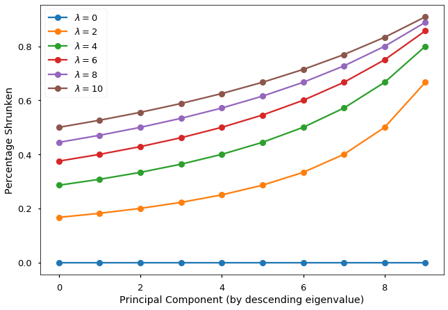
2. The shrinking effect of ridge regularization depends on both $\lambda$ and eigenvalues of the corresponding PC:
   • Larger $\lambda$ corresponds to heavier shrinking for every parameter.
   • However, given the same $\lambda$, principal components corresponding to larger eigenvalues receive the least shrinking.

To demonstrate the two shrinking effects, I plotted the percentage shrunken ($1- l_{i}/(l_{i}+\lambda)$) as a function of the ordered principal components as well as the value of the ridge regularization parameter. The two shrinking effects are clearly visible from this figure.

Result 1.2

It follows from Result 1.1 that we can establish a direct link between the OLS estimate $\hat{\boldsymbol{\beta}}$ and the ridge estimate $\boldsymbol{\beta}^*$ through spectral decomposition of the var-cov matrix. Specifically, we have

for $i=1, \ldots, p$.

Result 1.3

One measure of the quality of the estimators $\boldsymbol{\beta}^*$ is the trace mean square error (MSE):

Now, from the previous two results, we can show that the trace MSE of the ridge estimates can be decomposed into two parts: variance and bias, and obtain an explicit formula for them. The availability of the exact formula for MSE allows things like regularization path to be computed easily.

Specifically, we have

where the first component is the sum of variances:

and the second component is the sum of squared biases:

Result 1.4

This is a quick but revealing result that follows from Result 1.3. Taking a partial derivative of the trace MSE function with respect to $\lambda$ and take $\lambda = 0$, we get

Notice that the gradient of the trace MSE function is negative when $\lambda$ is 0. This tells us two things:

1. We can reduce the trace MSE by taking a non-zero $\lambda$ value. In particular, we are trading a bit of bias for a reduction in variance as the variance function ($\gamma_1$) is monotonically decreasing in $\lambda$. However, we need to find the right balance between variance and bias so that the overall trace MSE is minimized.
2. The reduction in trace MSE by ridge regularization is higher when some $l_i$s are small. That is, when there is considerable collinearity among the predictors, ridge regularization can achieve much smaller trace MSE than OLS.

Visualization

Using the sklearn.metrics.make_regression function, I generated a noisy regression data set with 50 samples and 10 features. However, most of the variances (in PCA sense) are explained by 5 of those 10 features, i.e. last 5 eigenvalues are relatively small. Here are the regularization path and the coefficient error plot.

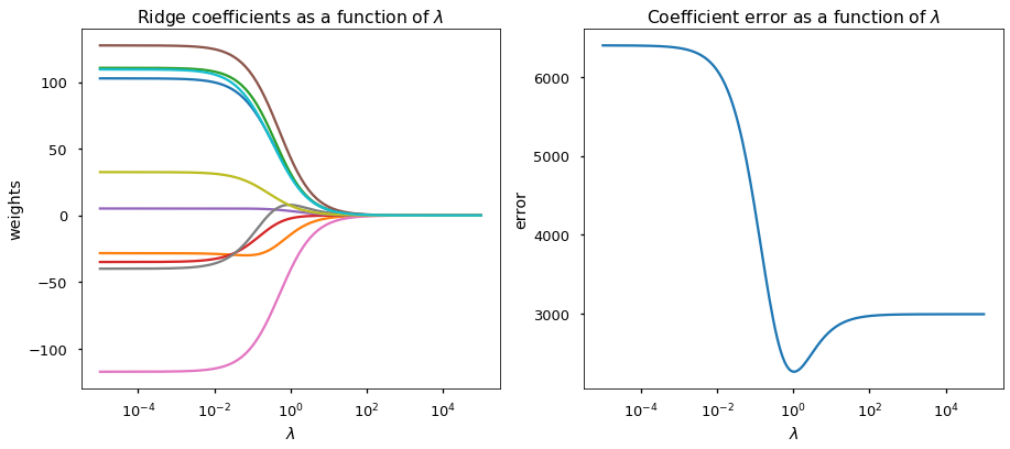
From the figure, we can clearly see that

• Increasing $\lambda$ shrinks every coefficient towards 0. 
• OLS procedure (left-hand side of both figures) produces erroneous (and with a large variance) estimate. the estimator MSE is significantly larger than that of the ridge regression. 
• An optimal $\lambda$ is found at around 1 where the MSE of ridge estimated coefficients is minimized. 
• On the other hand, $\lambda$ values larger and smaller than 1 are suboptimal as they lead to over-regularization and under-regularization in this case.

import numpy as np
import matplotlib.pyplot as plt
from sklearn.datasets import make_regression
from sklearn.linear_model import Ridge
from sklearn.metrics import mean_squared_error

clf = Ridge()

X, y, w = make_regression(n_samples=50, n_features=10, coef=True,
                          random_state=1, noise=50, 
                          effective_rank=5)

coefs = []
errors = []

lambdas = np.logspace(-5, 5, 200)

# Train the model with different regularisation strengths
for a in lambdas:
    clf.set_params(alpha=a)
    clf.fit(X, y)
    coefs.append(clf.coef_)
    errors.append(mean_squared_error(clf.coef_, w))

# Display results
with plt.style.context('seaborn-talk'):
    plt.figure(figsize=(15, 6))

    plt.subplot(121)
    ax = plt.gca()
    ax.plot(lambdas, coefs)
    ax.set_xscale('log')
    plt.xlabel('$\lambda$')
    plt.ylabel('weights')
    plt.title('Ridge coefficients as a function of $\lambda$')
    plt.axis('tight')

    plt.subplot(122)
    ax = plt.gca()
    ax.plot(lambdas, errors)
    ax.set_xscale('log')
    plt.xlabel('$\lambda$')
    plt.ylabel('error')
    plt.title('Coefficient error as a function of $\lambda$')
    plt.axis('tight')

    plt.show()

References