Expectation-maximization algorithm, explained

A comprehensive guide to the EM algorithm with intuitions, examples, Python implementation, and maths

Yes! Let’s talk about the expectation-maximization algorithm (EM, for short). If you are in the data science “bubble”, you’ve probably come across EM at some point in time and wondered: What is EM, and do I need to know it?

It’s the algorithm that solves Gaussian mixture models, a popular clustering approach. The Baum-Welch algorithm essential to hidden Markov models is a special type of EM. It works with both big and small data; it thrives when there is missing information while other techniques fail. It’s such a classic, powerful, and versatile statistical learning technique that it’s taught in almost all computational statistics classes. After reading this article, you could gain a strong understanding of the EM algorithm and know when and how to use it.

We start with two motivating examples (unsupervised learning and evolution). Next, we see what EM is in its general form. We jump back in action and use EM to solve the two examples. We then explain both intuitively and mathematically why EM works like a charm. Lastly, a summary of this article and some further topics are presented.

• Motivating examples: Why do we care?
• General framework: What is EM?
• EM in action: Does it really work?
• Explained: Why does it work?
• Summary
• Further topics

Motivating examples: Why do we care?

Maybe you already know why you want to use EM, or maybe you don’t. Either way, let me use two motivating examples to set the stage for EM. These are quite lengthy, I know, but they perfectly highlight the common feature of the problems that EM is best at solving: the presence of missing information.

Unsupervised learning: Solving Gaussian mixture model for clustering

Suppose you have a data set with $n$ number of data points. It could be a group of customers visiting your website (customer profiling) or an image with different objects (image segmentation). Clustering is the task of finding out $k$ natural groups for your data when you don’t know (or don’t specify) the real grouping. This is an unsupervised learning problem because no ground-truth labels are used.

Such clustering problem can be tackled by several types of algorithms, e.g., combinatorial type such as k-means or hierarchical type such as Ward’s hierarchical clustering. However, if you believe that your data could be better modeled as a mixture of normal distributions, you would go for Gaussian mixture model (GMM).

The underlying idea of GMM is that you assume there’s a data generating mechanism behind your data. This mechanism first chooses one of the $k$ normal distributions (with a certain probability) and then delivers a sample from that distribution. Therefore, once you have estimated each distribution’s parameters, you could easily cluster each data point by selecting the one that gives the highest likelihood.

FIGURE 1. An example of mixture of Gaussian data and clustering using k-means and GMM (solved by EM).

However, estimating the parameters is not a simple task since we do not know which distribution generated which points (missing information). EM is an algorithm that can help us solve exactly this problem. This is why EM is the underlying solver in scikit-learn’s GMM implementation.

Population genetics: Estimating moth allele frequencies to observe natural selection

Have you heard the phrase “industrial melanism” before? Biologists coined the term in the 19th century to describe how animals change their skin color due to the massive industrialization in the cities. They observed that previously rare dark peppered moths started to dominate the population in coal-fueled industrialized towns. Scientists at the time were surprised and fascinated by this observation. Subsequent research suggests that the industrialized cities tend to have darker tree barks that disguise darker moths better than the light ones. You can play this peppered moth game to understand the phenomenon better.

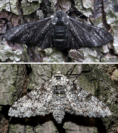
FIGURE 2. Dark (top) and light (bottom) peppered moth. Image by Jerzy Strzelecki via Wikimedia Commons

As a result, dark moths survive the predation better and pass on their genes, giving rise to a predominantly dark peppered moth population. To prove their natural selection theory, scientists first need to estimate the percentage of black-producing and light-producing genes/alleles present in the moth population. The gene responsible for the moth’s color has three types of alleles: C, I, and T. Genotypes CC, CI, and CT produce dark peppered moth (Carbonaria); TT produces light peppered moth (Typica); II and IT produce moths with intermediate color (Insularia).

Here’s a hand-drawn graph that shows the observed and missing information.

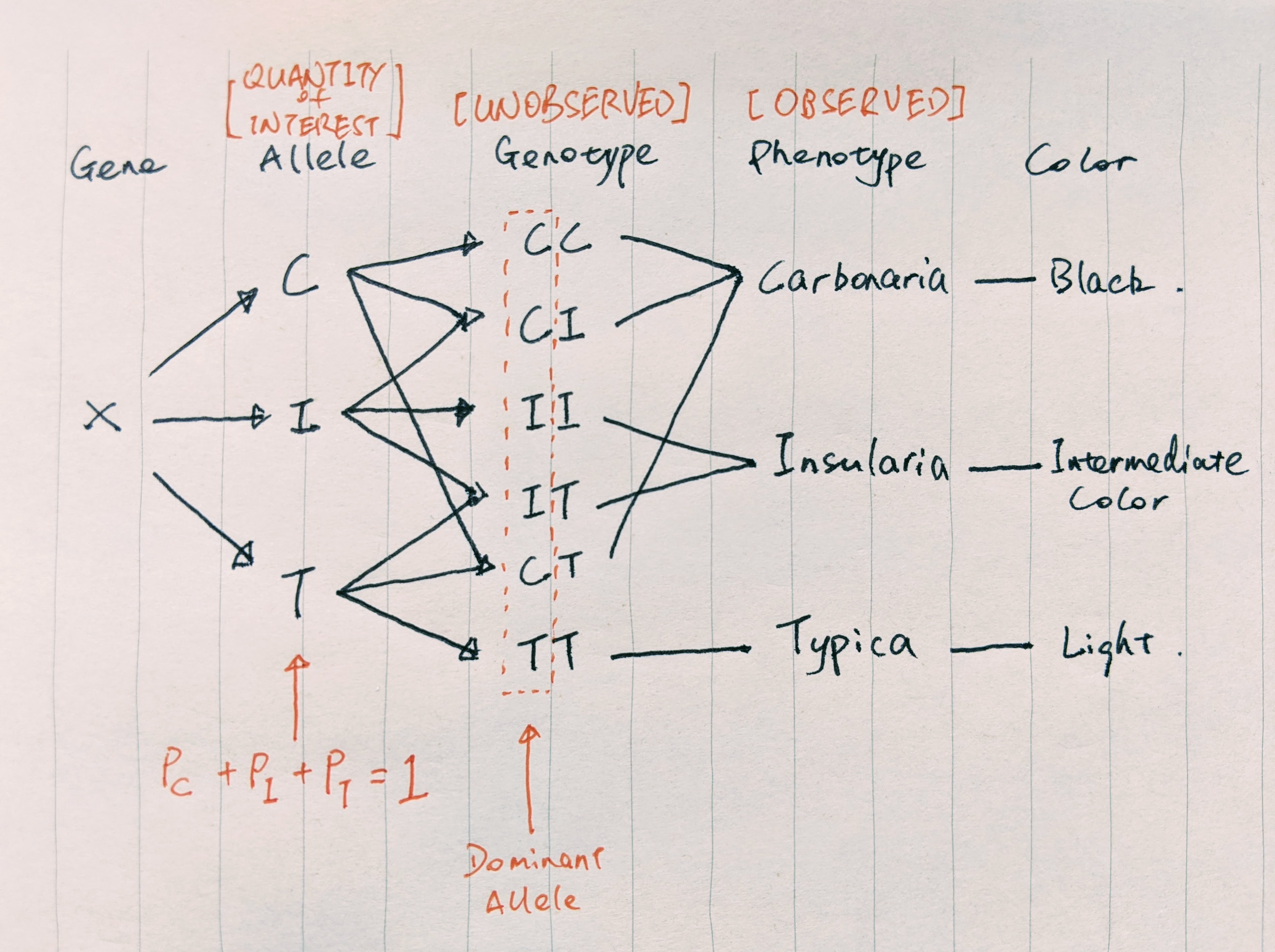FIGURE 3. Relationship between peppered moth alleles, genotypes, and phenotypes. We observed phenotypes, but wish to estimate percentages of alleles in the population. Image by author

We wish to know the percentages of C, I, and T in the population. However, we can only observe the number of Carbonaria, Typica, and Insularia moths by capturing them, but not the genotypes (missing information). The fact that we do not observe the genotypes and multiple genotypes produce the same subspecies make the calculation of the allele frequencies difficult. This is where EM comes in to play. With EM, we can easily estimate the allele frequencies and provide concrete evidence for the micro-evolution happening on a human time scale due to environmental pollution.

How does EM tackle the GMM problem and the peppered moth problem in the presence of missing information? We will illustrate these in the later section. But first, let’s see what EM is really about.

General framework: What is EM?

At this point, you must be thinking (I hope): All these examples are wonderful, but what is really EM? Let’s dive into it.

EM algorithm is an iterative optimization method that finds the maximum likelihood estimate (MLE) of parameters in problems where hidden/missing/latent variables are present. It was first introduced in its full generality by Dempster, Laird, and Rubin (1977) in their famous paper¹ (currently 62k citations). It has been widely used for its easy implementation, numerical stability, and robust empirical performance.

Let’s set up the EM for a general problem and introduce some notations. Suppose that $Y$ are our observed variables, $X$ are hidden variables, and we say that the pair $(X, Y)$ is the complete data. We also denote any unknown parameter of interest as $\theta \in \Theta$. The objective of most parameter estimation problems is to find the most probable $\theta$ given our model and data, i.e.,

where $p_\theta(\mathbf{y})$ is the incomplete-data likelihood. Using the law of total probability, we can also express the incomplete-data likelihood as

where $p_\theta(\mathbf{x}, \mathbf{y})$ is known as the complete-data likelihood.

What’s with all these complete- and incomplete-data likelihoods? In many problems, the maximization of the incomplete-data likelihood $p_\theta(\mathbf{y})$ is difficult because of the missing information. On the other hand, it’s often easier to work with complete-data likelihood. EM algorithm is designed to take advantage of this observation. It iterates between an expectation step (E-step) and a maximization step (M-step) to find the MLE.

Assuming $\theta^{(n)}$ is the estimate obtained at the $n$th iteration, the algorithm iterates between the two steps as follows:

• E-step: define $Q(\theta | \theta^{(n)})$ as the conditional expectation of the complete-data log-likelihood w.r.t. the hidden variables, given observed data and current parameter estimate, i.e.,

  \[\begin{align} \label{eqn:e_step} Q(\theta | \theta^{(n)}) = \mathbb{E}_{X|\mathbf{y}, \theta^{(n)}}\left[\ln p_\theta(\mathbf{x}, \mathbf{y})\right] \,. \end{align}\]

• M-step: find a new $\theta$ that maximizes the above expectation and set it to $\theta^{(n+1)}$, i.e.,

The above definitions might seem hard-to-grasp at first. Some intuitive explanation might help:

• E-step: This step is asking, given our observed data $\mathbf{y}$ and current parameter estimate $\theta^{(n)}$, what are the probabilities of different $X$? Also, under these probable $X$, what are the corresponding log-likelihoods?
• M-step: Here we ask, under these probable $X$, what is the value of $\theta$ that gives us the maximum expected log-likelihood?

The algorithm iterates between these two steps until a stopping criterion is reached, e.g., when either the Q function or the parameter estimate has converged. The entire process can be illustrated in the following flowchart.

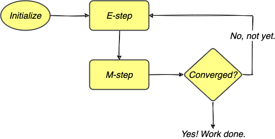
FIGURE 4. The EM algorithm iterates between E-step and M-step to obtain MLEs and stops when the estimates have converged. Image by author

That’s it! With two equations and a bunch of iterations, you have just unlocked one of the most elegant statistical inference techniques!

EM in action: Does it really work?

What we’ve seen above is the general framework of EM, not the actual implementation of it. In this section, we will see step-by-step just how EM is implemented to solve the two previously mentioned examples. After verifying that EM does work for these problems, we then see intuitively and mathematically why it works in the next section.

Solving GMM for clustering

Suppose we have some data and would like to model the density of them.

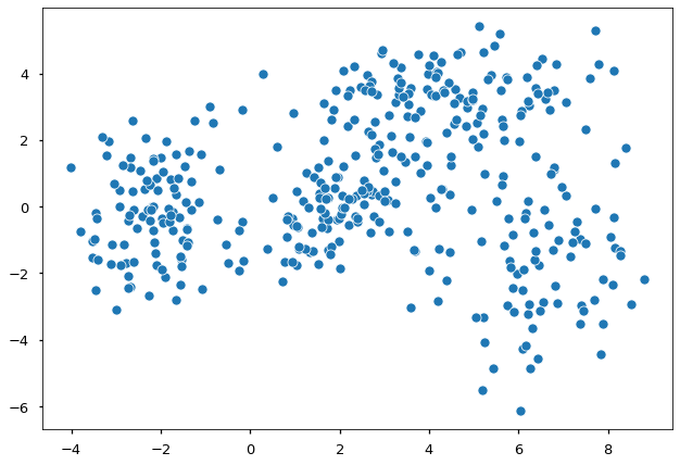FIGURE 5. 400 points generated as a mixture of four different normal distributions. Image by author

Are you able to see the different underlying distributions? Apparently, these data come from more than one distribution. Thus a single normal distribution would not be appropriate, and we use a mixture approach. In general, GMM-based clustering is the task of clustering $y_1, \dots, y_n$ data points into $k$ groups. We let

Thus, $x_i$ is the one-hot coding of data $y_i$, e.g., $x_i = [0, 0, 1]$ if $k = 3$ and $y_i$ is from group 3. In this case, the collection of data points $\mathbf{y}$ is the incomplete data, and $(\mathbf{x}, \mathbf{y})$ is the augmented complete data. We further assume that each group follows a normal distribution, i.e.,

Following the usual mixture Gaussian model set up, a new point is generated from the $k$th group with probability $P(x_{ik} = 1) = w_k$ and $\sum_{i=1}^{k} w_i = 1$. Suppose we are only working with the incomplete data $\mathbf{y}$. The likelihood of one data point under a GMM is

where $\phi(\cdot; \mu, \Sigma)$ is the PDF of a normal distribution with mean $\mu$ and variance-covariance $\Sigma$. The total log-likelihood of $n$ points is

In our problem, we are trying to estimate three groups of parameters: the group mixing probabilities ($\mathbf{w}$) and each distribution’s mean and covariance matrix ($\boldsymbol{\mu}, \boldsymbol{\Sigma}$). The usual approach to parameter estimation is by maximizing the above total log-likelihood function w.r.t. each parameter (MLE). However, this is difficult to do due to the summation inside the $\log$ term.

Expectation step

Let’s use the EM approach instead! Remember that we first need to define the Q function in the E-step, which is the conditional expectation of the complete-data log-likelihood. Since $(\mathbf{x}, \mathbf{y})$ is the complete data, the corresponding likelihood of one data point is

and only the term with $x_{ij} = 1$ is active. Hence, our total complete-data log-likelihood is

Denote $\theta$ as the collection of unknown parameters $(\mathbf{w}, \boldsymbol{\mu}, \boldsymbol{\Sigma})$, and $\theta^{(n)}$ as the estimates from the last iteration. Following the E-step formula in ($\ref{eqn:e_step}$), we obtain the Q function as

where

Here $z_{ij}^{(n)}$ is the probability that data $y_i$ is in class $j$ with the current parameter estimates $\theta^{(n)}$. This probability is also called responsibility in some texts. It means the responsibility of each class to this data point. It’s also a constant given the observed data and $\theta^{(n)}$.

Maximization step

Recall that the EM algorithm proceeds by iterating between the E-step and the M-step. We have obtained the latest iteration’s Q function in the E-step above. Next, we move on to the M-step and find a new $\theta$ that maximizes the Q function in ($\ref{eqn:gmm_e_step}$), i.e., we find

A closer look at the obtained Q function reveals that it’s actually a weighted normal distribution MLE problem. That means, the new $\theta$ has closed-form formulas and can be verified easily using differentiation:

for $j = 1, \dots, k$.

How does it perform?

We go back to the opening problem in this section. I simulated 400 points using four different normal distributions. FIGURE 5 is what we see if we do not know the underlying true groupings. We run the EM procedure as derived above and set the algorithm to stop when the log-likelihood does not change anymore.

In the end, we found the mixing probabilities and all four group’s means and covariance matrices. FIGURE 6 below shows the density contours of each distribution found by EM superimposed on the data, which are now color-coded by their ground-truth groupings. Both the locations (means) and the scales (covariances) of the four underlying normal distributions are correctly identified. Unlike k-means, EM gives us both the clustering of the data and the generative model (GMM) behind them.

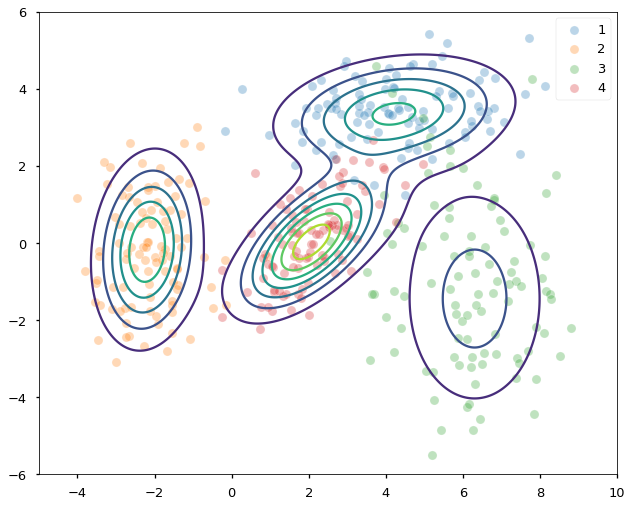FIGURE 6.  Density contours superimposed on samples from four different normal distributions. Image by author

  def em_gmm_vect(xs, pis, mus, sigmas, tol=0.01, max_iter=100):
    """
    EM algorithm implementation for solving Gaussian mixture model inference problem.

    Parameter:
    xs: n-by-p, observed data
    pis: 1-by-k, group mixing probabilities
    mus: k-by-p, mean vector of k groups
    sigmas: k-by-p-by-p, variance-covariance matrix of k groups
    
    Return:
    ll_new: maximum log-likelihood found
    pis, mus, sigmas: parameter results
    """
    
    n, p = xs.shape
    k = len(pis)
    
    ll_old = 0
    
    for i in range(max_iter):
        ll_new = 0
    
        # E-step
        ws = np.zeros((k, n))
        for j in range(k):
            ws[j, :] = pis[j] * mvn(mus[j], sigmas[j]).pdf(xs)
        ws /= ws.sum(0)
    
        # M-step
        pis = ws.sum(axis=1)
        pis /= n
        
        pis_hist.append(pis)
    
        mus = np.dot(ws, xs)
        mus /= ws.sum(1)[:, None]
    
        sigmas = np.zeros((k, p, p))
        for j in range(k):
            ys = xs - mus[j, :]
            sigmas[j] = (ws[j,:,None,None] * mm(ys[:,:,None], ys[:,None,:])).sum(axis=0)
        sigmas /= ws.sum(axis=1)[:,None,None]
    
        # update complete log likelihood
        ll_new = 0
        for pi, mu, sigma in zip(pis, mus, sigmas):
            ll_new += pi*mvn(mu, sigma).pdf(xs)
        ll_new = np.log(ll_new).sum()
    
        if np.abs(ll_new - ll_old) < tol:
            break
        ll_old = ll_new
    
    return ll_new, pis, mus, sigmas

import numpy as np
import matplotlib.pyplot as plt
import seaborn as sns
from scipy.stats import multivariate_normal as mvn
from numpy.core.umath_tests import matrix_multiply as mm

np.random.seed(123)

# create data set
n = 400
_mus = np.array([[4,3.5], 
                 [-2,0], 
                 [6, -1],
                 [2,0]])
_sigmas = np.array([[[3, 0.2], [0, 0.5]], 
                    [[1, 0],[0.2,2]], 
                    [[2,0],[0,-4]], 
                    [[1,.6],[.6,1]]])

_pis = np.array([0.25]*_mus.shape[0])
xs = np.concatenate([np.random.multivariate_normal(mu, sigma, int(pi*n))
                    for pi, mu, sigma in zip(_pis, _mus, _sigmas)])

# visualize data without labels
with plt.style.context('seaborn-talk'):
    sns.scatterplot(xs[:,0], xs[:, 1])
    plt.show()
    
# initial guesses for parameters
pis = np.random.random(4)
pis /= pis.sum()  # normalize
mus = np.random.random((4,2))
sigmas = np.array([np.eye(2)] * 4)

# run EM
# remember to include em_gmm_vect function
ll2, pis2, mus2, sigmas2 = em_gmm_vect(xs, pis, mus, sigmas)

# visualize results
intervals = 1000
ys = np.linspace(-6,10,intervals)
X, Y = np.meshgrid(ys, ys)
_ys = np.vstack([X.ravel(), Y.ravel()]).T

z = np.zeros(len(_ys))
for pi, mu, sigma in zip(pis2, mus2, sigmas2):
    z += pi*mvn(mu, sigma).pdf(_ys)
z = z.reshape((intervals, intervals))

with plt.style.context('seaborn-talk'):
    ax = plt.subplot(111)
    sns.scatterplot(xs[:100,0], xs[:100, 1], alpha=.3)
    sns.scatterplot(xs[100:200,0], xs[100:200, 1], alpha=.3)
    sns.scatterplot(xs[200:300,0], xs[200:300, 1], alpha=.3)
    sns.scatterplot(xs[300:,0], xs[300:, 1], alpha=.3)
    plt.legend(['1', '2', '3', '4'])
    plt.contour(X, Y, z)
    plt.axis([-5,10,-6,6])
    ax.axes.set_aspect('equal')
    plt.tight_layout()

Estimating allele frequencies

We return to the population genetics problem mentioned earlier. Suppose we captured $n$ moths and of which there are three different types: Carbonaria, Typica, and Insularia. However, we do not know the genotype of each moth except for Typica moths, see FIGURE 3 above. We wish to estimate the population allele frequencies. Let’s speak in EM terms. Here’s what we know:

• Observed:
  • $X = (n_{\mathrm{Car}}, n_{\mathrm{Typ}}, n_{\mathrm{Ins}})$
• Unobserved: the number of different genotypes
  • $Y = (n_{\mathrm{CC}}, n_{\mathrm{CI}}, n_{\mathrm{CT}}, n_{\mathrm{II}}, n_{\mathrm{IT}}, n_{\mathrm{TT}})$
• But we do know the relationship between them:
  • $n_{\mathrm{Car}} = n_{\mathrm{CC}} + n_{\mathrm{CI}} + n_{\mathrm{CT}}$
  • $n_{\mathrm{Typ}} = n_{\mathrm{TT}}$
  • $n_{\mathrm{Ins}} = n_{\mathrm{II}} + n_{\mathrm{IT}}$
• Parameter of interest: allele frequencies
  • $\theta = (p_\mathrm{C}, p_\mathrm{I}, p_\mathrm{T})$
  • and we know $p_\mathrm{C} + p_\mathrm{I} + p_\mathrm{T} = 1$

There’s another important modeling principle that we need to use: the Hardy–Weinberg principle, which says that the genotype frequency is the product of the corresponding allele frequency or double that when the two alleles are different. That is, we can expect the genotype frequencies of $n_{\mathrm{CC}}, n_{\mathrm{CI}}, n_{\mathrm{CT}}, n_{\mathrm{II}}, n_{\mathrm{IT}}, n_{\mathrm{TT}}$ to be

Good! Now we are ready to plug in the EM framework. What’s the first step?

Expectation step

Just like the GMM case, we first need to figure out the complete-data likelihood. Notice that this is actually a multinomial distribution problem. We have a population of moths, the chance of capturing a moth of genotype $\mathrm{CC}$ is $p_{\mathrm{C}}^2$, similarly for the other genotypes. Therefore, the complete-data likelihood is just the multinomial distribution PDF:

And the complete-data log-likelihood can be written in the following decomposed form:

Remember that the E-step is taking a conditional expectation of the above likelihood w.r.t. the unobserved data $Y$, given the latest iteration’s parameter estimates $\theta^{(n)}$. The Q function is found to be

where $n_{\mathrm{CC}}^{(n)}$ is expected number of $\mathrm{CC}$ type moth given the current allele frequency estimates, and similarly for the other types. $k(\cdot)$ is a function that does not involve $\theta$.

Maximization step

Since we obtained the expected number of each phenotype, e.g. $n_{\mathrm{CC}}^{(n)}, n_{\mathrm{CI}}^{(n)}$, estimating the allele frequencies is easy. Intuitively, the frequency of allele $\mathrm{C}$ is calculated as the ratio between the number of allele $\mathrm{C}$ present in the population and the total number of alleles. This works for the other alleles as well. Therefore, in the M-step, we obtain

In fact, we could obtain the same M-step formulas by differentiating the Q function and setting them to zero (usual optimization routine).

How does it perform?

Let’s try solving the peppered moth problem using the above derived EM procedure. Suppose we captured 622 peppered moths. 85 of them are Carbonaria, 196 of them are Insularia, and 341 of them are Typica. We run the EM iterations for 10 steps, FIGURE 7 shows that we obtain converged results in less than five steps.

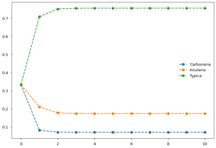FIGURE 7.  EM algorithm converges in less than five steps and finds the allele frequencies. Image by author

import matplotlib.pyplot as plt

def e_step(n_car, n_ins, n_typ, p_C, p_I, p_T):
    
    CC_prob = p_C*p_C
    CI_prob = 2*p_C*p_I
    CT_prob = 2*p_C*p_T
    
    II_prob = p_I*p_I
    IT_prob = 2*p_I*p_T
    
    C_prob = CC_prob + CI_prob + CT_prob
    I_prob = II_prob + IT_prob
    
    n_CC = n_car * CC_prob/C_prob
    n_CI = n_car * CI_prob/C_prob
    n_CT = n_car * CT_prob/C_prob
    n_II = n_ins * II_prob/I_prob
    n_IT = n_ins * IT_prob/I_prob
    n_TT = n_typ
    
    return (n_CC, n_CI, n_CT, n_II, n_IT, n_TT)
        
def m_step(n, n_CC, n_CI, n_CT, n_II, n_IT, n_TT):
    
    p_C = (2*n_CC + n_CI + n_CT)/(2*n)
    p_I = (2*n_II + n_IT)/(2*n)
    p_T = 1 - p_C - p_I
    
    return (p_C, p_I, p_T)

# Given observed information
nC = 85
nI = 196
nT = 341
n = nC + nI + nT

# Initialize
p_C = 1/3
p_I = 1/3
p_T = 1/3

# Record history for visualization
hist = []
hist.append([p_C, p_I, p_T])

for i in range(10):
    # E-step
    n_CC, n_CI, n_CT, n_II, n_IT, n_TT = e_step(nC, nI, nT, p_C, p_I, p_T)
    
    # M-step
    p_C, p_I, p_T = m_step(n, n_CC, n_CI, n_CT, n_II, n_IT, n_TT)
    
    hist.append([p_C, p_I, p_T])

with plt.style.context('seaborn-talk'):
    plt.plot(hist, 'o--')
    plt.legend(['Carbonaria', 'Insularia', 'Typica'])
    plt.tight_layout()

What did we learn from the examples?

Estimating the allele frequencies is difficult because of the missing phenotype information. EM helps us to solve this problem by augmenting the process with exactly the missing information. If we look back at the E-step and M-step, we see that the E-step calculates the most probable phenotype counts given the latest frequency estimates; the M-step then calculates the most probable frequencies given the latest phenotype count estimates. This process is evident in the GMM problem as well: the E-step calculates the class responsibilities for each data given the current class parameter estimates; the M-step then estimates the new class parameters using those responsibilities as the data weights.

Explained: Why does it work?

Working through the previous two examples, we see clearly that the essence of EM lies in the E-step/M-step iterative process that augments the observed information with the missing information. And we see that it indeed finds the MLEs effectively. But why does this iterative process work? Is EM just a smart hack, or is it well-supported by theory? Let’s find out.

Intuitive explanation

We start by gaining an intuitive understanding of why EM works. EM solves the parameter estimation problem by transferring the task of maximizing incomplete-data likelihood to maximizing complete-data likelihood in some small steps.

Imagine you are hiking up Mt. Fuji 🗻 for the first time. There are nine stations to reach before the summit, but you do not know the route. Luckily, there are hikers coming down from the top, and they can give you a rough direction to the next station. Therefore, here’s what you can do to reach the top: start at the base station and ask people for the direction to the second station; go to the second station and ask the people there for the path to the third station, and so on. At the end of the day (or start of the day, if you are catching sunrise 🌄), there’s a high chance you’ll reach the summit.

That’s very much what EM does to find the MLEs for problems where we have missing data. Instead of maximizing $\ln p(\mathbf{x})$ (find the route to summit), EM maximizes the Q function and finds the next $\theta$ that also increases $\ln p(\mathbf{x})$ (ask direction to the next station). FIGURE 8 below illustrates this process in two iterations. Note that the G function is just a combination of Q function and a few other terms constant w.r.t. $\theta$. Maximizing G function w.r.t. $\theta$ is equivalent to maximizing Q function.

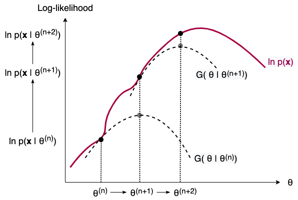FIGURE 8.  The iterative process of EM illustrated in two steps. As we build and maximize a G function (equivalently, Q function) from the current parameter estimate, we obtain the next parameter estimate. In the process, the incomplete-data log-likelihood is also increased. Image by author

Summary

In this article, we see that EM converts a difficult problem with missing information to an easy problem through the optimization transfer framework. We also see EM in action by solving step-by-step two problems with Python implementation (Gaussian mixture clustering and peppered moth population genetics). More importantly, we show that EM is not just a smart hack but has solid mathematical groundings on why it would work.

I hope this introductory article has helped you a little in getting to know the EM algorithm. From here, if you are interested, consider exploring the following topics.

Further topics

Digging deeper, the first question you might ask is: So, is EM perfect? Of course, it’s not. Sometimes, the Q function is difficult to obtain analytically. We could use Monte Carlo techniques to estimate the Q function, e.g., check out Monte Carlo EM. Sometimes, even with complete-data information, the Q function is still difficult to maximize. We could consider alternative maximizing techniques, e.g., see expectation conditional maximization (ECM). Another disadvantage of EM is that it provides us with only point estimates. In case we want to know the uncertainty in these estimates, we would need to conduct variance estimation through other techniques, e.g., Louis’s method, supplemental EM, or bootstrapping.

Thanks for reading! Please consider leaving feedback for me below.

References